Xhistogram Tutorial
Histograms are the foundation of many forms of data analysis. The goal of xhistogram is to make it easy to calculate weighted histograms in multiple dimensions over n-dimensional arrays, with control over the axes. Xhistogram builds on top of xarray, for automatic coordiantes and labels, and dask, for parallel scalability.
Toy Data
We start by showing an example with toy data. First we use xarray to create some random, normally distributed data.
1D Histogram
[1]:
import xarray as xr
import numpy as np
%matplotlib inline
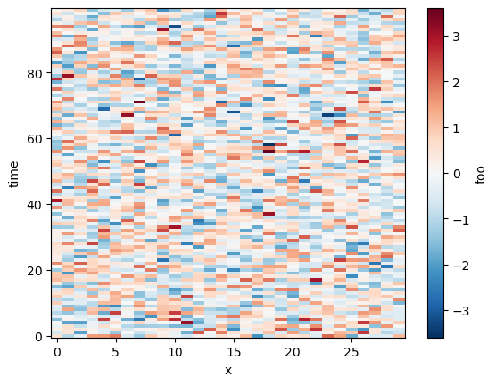
nt, nx = 100, 30
da = xr.DataArray(np.random.randn(nt, nx), dims=['time', 'x'],
name='foo') # all inputs need a name
display(da)
da.plot()
Matplotlib is building the font cache; this may take a moment.
<xarray.DataArray 'foo' (time: 100, x: 30)>
array([[ 0.50860314, -1.0165478 , -0.32705033, ..., -0.51147417,
        -0.41292428,  1.12693927],
       [-0.62873018,  0.48770407, -1.94717808, ...,  0.45863088,
        -1.01518664, -0.77006161],
       [ 0.20045831,  0.52220286,  0.37111314, ...,  0.45354817,
        -0.4637895 , -0.55069174],
       ...,
       [-0.43713369,  0.19003816, -0.80609825, ..., -0.53770166,
         1.97766153, -0.1327787 ],
       [ 0.51990755, -0.7327349 ,  0.136738  , ..., -1.71930054,
        -0.52837142,  0.81463048],
       [ 0.04648285,  0.30396924,  0.81445339, ..., -0.70200964,
        -0.93409991,  0.75207502]])
Dimensions without coordinates: time, x[1]:
<matplotlib.collections.QuadMesh at 0x7f8dbfcca4c0>
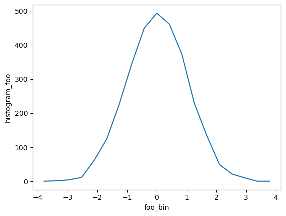
By default xhistogram operates on all dimensions of an array, just like numpy. However, it operates on xarray DataArrays, taking labels into account.
[2]:
from xhistogram.xarray import histogram

bins = np.linspace(-4, 4, 20)
h = histogram(da, bins=[bins])
display(h)
h.plot()
<xarray.DataArray 'histogram_foo' (foo_bin: 19)>
array([  1,   2,   5,  12,  62, 124, 226, 344, 449, 493, 461, 373, 229,
       134,  50,  22,  11,   1,   1])
Coordinates:
* foo_bin (foo_bin) float64 -3.789 -3.368 -2.947 -2.526 ... 2.947 3.368 3.789[2]:
[<matplotlib.lines.Line2D at 0x7f8dbfb99fa0>]
TODO: - Bins needs to be a list; this is annoying, would be good to accept single items - The foo_bin coordinate is the estimated bin center, not the bounds. We need to add the bounds to the coordinates, but we can as long as we are returning DataArray and not Dataset.
Both of the above need GitHub Issues
Histogram over a single axis
[3]:
h_x = histogram(da, bins=[bins], dim=['time'])
h_x.plot()
[3]:
<matplotlib.collections.QuadMesh at 0x7f8dbfaca790>
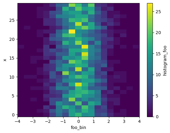
TODO: - Relax / explain requirement that dims is always a list
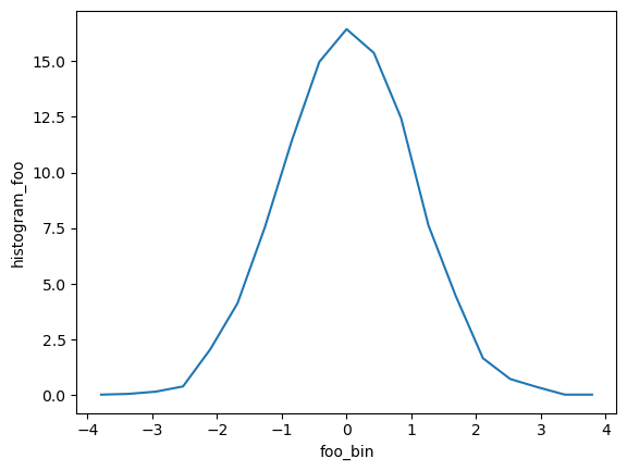
[4]:
h_x.mean(dim='x').plot()
[4]:
[<matplotlib.lines.Line2D at 0x7f8dbfa09610>]
Weighted Histogram
Weights can be the same shape as the input:
[5]:
weights = 0.4 * xr.ones_like(da)
histogram(da, bins=[bins], weights=weights)
[5]:
<xarray.DataArray 'histogram_foo' (foo_bin: 19)>
array([  0.4,   0.8,   2. ,   4.8,  24.8,  49.6,  90.4, 137.6, 179.6,
       197.2, 184.4, 149.2,  91.6,  53.6,  20. ,   8.8,   4.4,   0.4,
         0.4])
Coordinates:
* foo_bin (foo_bin) float64 -3.789 -3.368 -2.947 -2.526 ... 2.947 3.368 3.789Or can use Xarray broadcasting:
[6]:
weights = 0.2 * xr.ones_like(da.x)
histogram(da, bins=[bins], weights=weights)
[6]:
<xarray.DataArray 'histogram_foo' (foo_bin: 19)>
array([ 0.2,  0.4,  1. ,  2.4, 12.4, 24.8, 45.2, 68.8, 89.8, 98.6, 92.2,
       74.6, 45.8, 26.8, 10. ,  4.4,  2.2,  0.2,  0.2])
Coordinates:
* foo_bin (foo_bin) float64 -3.789 -3.368 -2.947 -2.526 ... 2.947 3.368 3.7892D Histogram
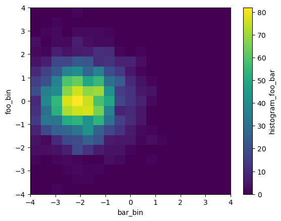
Now let’s say we have multiple input arrays. We can calculate their joint distribution:
[7]:
db = xr.DataArray(np.random.randn(nt, nx), dims=['time', 'x'],
                  name='bar') - 2

histogram(da, db, bins=[bins, bins]).plot()
[7]:
<matplotlib.collections.QuadMesh at 0x7f8dbf991760>
Real Data Example
Ocean Volume Census in TS Space
Here we show how to use xhistogram to do a volume census of the ocean in Temperature-Salinity Space
First we open the World Ocean Atlas dataset from the opendap dataset (http://apdrc.soest.hawaii.edu/dods/public_data/WOA/WOA13/1_deg/annual).
Here we read the annual mean Temparature, Salinity and Oxygen on a 5 degree grid.
[8]:
# Read WOA using opendap
Temp_url = 'http://apdrc.soest.hawaii.edu:80/dods/public_data/WOA/WOA13/5_deg/annual/temp'
Salt_url = 'http://apdrc.soest.hawaii.edu:80/dods/public_data/WOA/WOA13/5_deg/annual/salt'
Oxy_url = 'http://apdrc.soest.hawaii.edu:80/dods/public_data/WOA/WOA13/5_deg/annual/doxy'

ds = xr.merge([
    xr.open_dataset(Temp_url).tmn.load(),
    xr.open_dataset(Salt_url).smn.load(),
    xr.open_dataset(Oxy_url).omn.load()])
ds
/home/docs/checkouts/readthedocs.org/user_builds/xhistogram/conda/latest/lib/python3.9/site-packages/xarray/coding/times.py:150: SerializationWarning: Ambiguous reference date string: 1-1-1 00:00:0.0. The first value is assumed to be the year hence will be padded with zeros to remove the ambiguity (the padded reference date string is: 0001-1-1 00:00:0.0). To remove this message, remove the ambiguity by padding your reference date strings with zeros.
  warnings.warn(warning_msg, SerializationWarning)
/home/docs/checkouts/readthedocs.org/user_builds/xhistogram/conda/latest/lib/python3.9/site-packages/xarray/coding/times.py:201: CFWarning: this date/calendar/year zero convention is not supported by CF
  cftime.num2date(num_dates, units, calendar, only_use_cftime_datetimes=True)
/home/docs/checkouts/readthedocs.org/user_builds/xhistogram/conda/latest/lib/python3.9/site-packages/xarray/coding/times.py:682: SerializationWarning: Unable to decode time axis into full numpy.datetime64 objects, continuing using cftime.datetime objects instead, reason: dates out of range
  dtype = _decode_cf_datetime_dtype(data, units, calendar, self.use_cftime)
/home/docs/checkouts/readthedocs.org/user_builds/xhistogram/conda/latest/lib/python3.9/site-packages/numpy/core/_asarray.py:83: SerializationWarning: Unable to decode time axis into full numpy.datetime64 objects, continuing using cftime.datetime objects instead, reason: dates out of range
  return array(a, dtype, copy=False, order=order)
[8]:
<xarray.Dataset>
Dimensions:  (time: 1, lev: 102, lat: 36, lon: 72)
Coordinates:
  * time     (time) object -001-01-15 00:00:00
  * lev      (lev) float64 0.0 5.0 10.0 15.0 ... 5.2e+03 5.3e+03 5.4e+03 5.5e+03
  * lat      (lat) float64 -87.5 -82.5 -77.5 -72.5 -67.5 ... 72.5 77.5 82.5 87.5
  * lon      (lon) float64 -177.5 -172.5 -167.5 -162.5 ... 167.5 172.5 177.5
Data variables:
    tmn      (time, lev, lat, lon) float32 nan nan nan nan ... nan nan nan nan
    smn      (time, lev, lat, lon) float32 nan nan nan nan ... nan nan nan nan
    omn      (time, lev, lat, lon) float32 nan nan nan nan ... nan nan nan nan
Attributes:
long_name: statistical mean sea water temperature [degc] Use histogram to bin data points. Use canonical ocean T/S ranges, and bin size of \(0.1^0C\), and \(0.025psu\). Similar ranges and bin size as this review paper on Mode Waters: https://doi.org/10.1016/B978-0-12-391851-2.00009-X .
[9]:
sbins = np.arange(31,38, 0.025)
tbins = np.arange(-2, 32, 0.1)
[10]:
# histogram of number of data points
# histogram of number of data points
hTS = histogram(ds.smn, ds.tmn, bins=[sbins, tbins])
np.log10(hTS.T).plot(levels=31)
/home/docs/checkouts/readthedocs.org/user_builds/xhistogram/conda/latest/lib/python3.9/site-packages/xarray/core/computation.py:771: RuntimeWarning: divide by zero encountered in log10
  result_data = func(*input_data)
[10]:
<matplotlib.collections.QuadMesh at 0x7f8dbf647b50>
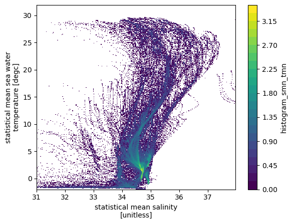
However, we would like to do a volume census, which requires the data points to be weighted by volume of the grid box.
\begin{equation} dV = dz*dx*dy \end{equation}
[11]:
# histogram of number of data points weighted by volume resolution
# Note that depth is a non-uniform axis

# Create a dz variable
dz = np.diff(ds.lev)
dz =np.insert(dz, 0, dz[0])
dz = xr.DataArray(dz, coords= {'lev':ds.lev}, dims='lev')

# weight by volume of grid cell (resolution = 5degree, 1degree=110km)
dVol = dz * (5*110e3) * (5*110e3*np.cos(ds.lat*np.pi/180))

# Note: The weights are automatically broadcast to the right size
hTSw = histogram(ds.smn, ds.tmn, bins=[sbins, tbins], weights=dVol)
np.log10(hTSw.T).plot(levels=31, vmin=11.5, vmax=16, cmap='brg')
[11]:
<matplotlib.collections.QuadMesh at 0x7f8dbe58d910>
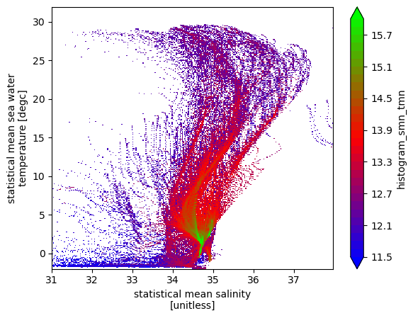
The ridges of this above plot are indicative of T/S classes with a lot of volume, and some of them are indicative of Mode Waters (example Eighteen Degree water with T\(\sim18^oC\), and S\(\sim36.5psu\).
Averaging a variable
Next we calculate the mean oxygen value in each TS bin.
\begin{equation} \overline{A} (m,n) = \frac{\sum_{T(x,y,z)=m, S(x,y,z)=n} (A(x,y,z) dV)}{\sum_{T(x,y,z)=m, S(x,y,z)=n}dV}. \end{equation}
[12]:
hTSO2 = (histogram(ds.smn.where(~np.isnan(ds.omn)),
                   ds.tmn.where(~np.isnan(ds.omn)),
                   bins=[sbins, tbins],
                   weights=ds.omn.where(~np.isnan(ds.omn))*dVol)/
                histogram(ds.smn.where(~np.isnan(ds.omn)),
                          ds.tmn.where(~np.isnan(ds.omn)),
                          bins=[sbins, tbins],
                          weights=dVol))

(hTSO2.T).plot(vmin=1, vmax=8)
[12]:
<matplotlib.collections.QuadMesh at 0x7f8dbe4c88b0>
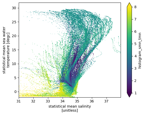
Some interesting patterns in average oxygen emerge. Convectively ventilated cold water have the highest oxygen and mode waters have relatively high oxygen. Oxygen minimum zones are interspersed in the middle of volumetic ridges (high volume waters).
NOTE: NaNs in weights will make the weighted sum as nan. To avoid this, call .fillna(0.) on your weights input data before calling histogram().
Dask Integration
Should just work, but need examples.